Classification with FACET: Prediabetes Study#
FACET is composed of the following key components:
Model Inspection
FACET introduces a new algorithm to quantify dependencies and interactions between features in ML models. This new tool for human-explainable AI adds a new, global perspective to the observation-level explanations provided by the popular SHAP approach. To learn more about FACET’s model inspection capabilities, see the getting started example below.
Model Simulation
FACET’s model simulation algorithms use ML models for virtual experiments to help identify scenarios that optimise predicted outcomes. To quantify the uncertainty in simulations, FACET utilises a range of bootstrapping algorithms including stationary and stratified bootstraps. For an example of FACET’s bootstrap simulations, see the getting started example below.
Enhanced Machine Learning Workflow
FACET offers an efficient and transparent machine learning workflow, enhancing scikit-learn’s tried and tested pipelining paradigm with new capabilities for model selection, inspection, and simulation. FACET also introduces sklearndf, an augmented version of scikit-learn with enhanced support for pandas dataframes that ensures end-to-end traceability of features.
Context
Prediabetes is a treatable condition that leads to many health complications and eventually type 2 diabetes. Identification of individuals at risk of prediabetes can improve early intervention and provide insights into those interventions that work best. Using a cohort of healthy (n=2847) and prediabetic (n=1509) patients derived from the NHANES 2013-14 U.S. cross-sectional survey we aim to create a classifier for prediabetes. For further details on data sources, definitions and the study cohort please see the Appendix (Data source and study cohort).
Utilizing FACET, we will do the following:
create a pipeline to find identify a well-performing classifier.
perform model inspection and simulation to gain understanding and insight into key factors predictive of prediabetes.
Tutorial outline
Required imports#
In order to run this notebook, we will import not only the FACET package, but also other packages useful to solve this task. Overall, we can break down the imports into three categories:
Common packages (pandas, matplotlib, etc.)
Required FACET classes (inspection, selection, validation, simulation, etc.)
Other BCG GAMMA packages which simplify pipelining (sklearndf, see on GitHub) and support visualization (pytools, see on GitHub) when using FACET
Common package imports
[2]:
import numpy as np
import pandas as pd
import matplotlib.pyplot as plt
from scipy import stats
import shap
import seaborn as sns
from sklearn.compose import make_column_selector
from sklearn.model_selection import RepeatedKFold, RandomizedSearchCV
FACET imports
[3]:
from facet.data import Sample
from facet.inspection import LearnerInspector
from facet.selection import LearnerSelector, ParameterSpace
from facet.validation import BootstrapCV
from facet.data.partition import ContinuousRangePartitioner
from facet.simulation import UnivariateProbabilitySimulator
from facet.simulation.viz import SimulationDrawer
sklearndf imports
Instead of using the “regular” scikit-learn package, we are going to use sklearndf (see on GitHub). sklearndf is an open source library designed to address a common issue with scikit-learn: the outputs of transformers are numpy arrays, even when the input is a data frame. However, to inspect a model it is essential to keep track of the feature names. sklearndf retains all the functionality available through scikit-learn plus the feature
traceability and usability associated with Pandas data frames. Additionally, the names of all your favourite scikit-learn functions are the same except for DF on the end. For example, the standard scikit-learn import:
from sklearn.pipeline import Pipeline
becomes:
from sklearndf.pipeline import PipelineDF
[4]:
from sklearndf.pipeline import PipelineDF, ClassifierPipelineDF
from sklearndf.classification import RandomForestClassifierDF
from sklearndf.classification.extra import LGBMClassifierDF
from sklearndf.transformation import (
    ColumnTransformerDF,
    OneHotEncoderDF,
    SimpleImputerDF,
)
from sklearndf.transformation.extra import BorutaDF
pytools imports
pytools (see on GitHub) is an open source library containing general machine learning and visualization utilities, some of which are useful for visualising the advanced model inspection capabilities of FACET.
[5]:
from pytools.viz.dendrogram import DendrogramDrawer
from pytools.viz.matrix import MatrixDrawer
Preprocessing and initial feature selection#
First we need to load our prediabetes data and create a simple preprocessing pipeline. For those interested some initial EDA can be found in the Appendix (Exploratory Data Analysis).
[6]:
# load the prepared data frame
prediab_df = pd.read_csv("pre_diab_nhanes.csv")

# create a couple of new interesting features
prediab_df["SBP_to_DBP"] = prediab_df["Average_SBP"] / prediab_df["Average_DBP"]
prediab_df["Waist_to_hgt"] = (
    prediab_df["Waist_Circumference"] / prediab_df["Standing_Height"]
)

# make clear based on dtypes these two features are categorical
prediab_df["General_health"] = prediab_df["General_health"].astype("object")
prediab_df["Healthy_diet"] = prediab_df["Healthy_diet"].astype("object")

# have a look
prediab_df.head().T
[6]:
| 0 | 1 | 2 | 3 | 4 | |
|---|---|---|---|---|---|
| Age | 73.0 | 56.0 | 61.0 | 56.0 | 65.0 |
| Gender | 2.0 | 1.0 | 2.0 | 2.0 | 1.0 |
| Waist_Circumference | NaN | 123.1 | 110.8 | 85.5 | 93.7 |
| Weight | 52.0 | 105.0 | 93.4 | 61.8 | 65.3 |
| Standing_Height | 162.4 | 158.7 | 161.8 | 152.8 | 172.4 |
| BMI | 19.7 | 41.7 | 35.7 | 26.5 | 22.0 |
| Average_SBP | 137.333333 | 157.333333 | 122.666667 | 122.0 | 141.333333 |
| Average_DBP | 86.666667 | 82.0 | 80.666667 | 72.666667 | 77.333333 |
| HDL_Cholesterol | 85.0 | 38.0 | 58.0 | 59.0 | 79.0 |
| Total_Cholesterol | 201.0 | 226.0 | 168.0 | 278.0 | 173.0 |
| High_BP | 1.0 | 1.0 | 1.0 | 0.0 | 0.0 |
| Sleep_hours | 9.0 | 5.0 | 9.0 | 6.0 | 7.0 |
| Trouble_sleeping | 0.0 | 0.0 | 0.0 | 1.0 | 0.0 |
| Sleep_disorder | 0.0 | 1.0 | 1.0 | 0.0 | 0.0 |
| Told_overweight | 0.0 | 1.0 | 1.0 | 0.0 | 0.0 |
| General_health | 5.0 | 5.0 | 3.0 | 3.0 | 3.0 |
| Family_hist_diab | 0 | 0 | 0 | 0 | 0 |
| Feel_at_risk_diab | 0.0 | 1.0 | 1.0 | 0.0 | 0.0 |
| Vigorous_work_activity | 0.0 | 1.0 | 0.0 | 1.0 | 1.0 |
| Moderate_work_activity | 1.0 | 0.0 | 0.0 | 1.0 | 0.0 |
| Walk_or_bicycle | 0.0 | 0.0 | 0.0 | 0.0 | 0.0 |
| Vigorous_rec_activity | 0.0 | 0.0 | 0.0 | 0.0 | 0.0 |
| Moderate_rec_activity | 0.0 | 0.0 | 0.0 | 0.0 | 0.0 |
| Tried_weight_loss_past_year | 0.0 | 1.0 | 1.0 | 0.0 | 0.0 |
| Healthy_diet | 2.0 | 5.0 | 4.0 | 2.0 | 3.0 |
| WBC_count | 6.6 | 9.4 | 5.2 | 9.5 | 6.3 |
| RBC_count | 4.72 | 4.93 | 4.66 | 4.43 | 4.35 |
| Hematocrit | 43.8 | 41.5 | 39.8 | 41.4 | 43.1 |
| Triglycerides | 88.0 | 327.0 | 68.0 | 262.0 | 39.0 |
| Uric_acid | 4.2 | 9.1 | 5.1 | 3.5 | 6.3 |
| Osmolality | 290.0 | 287.0 | 281.0 | 277.0 | 281.0 |
| Sodium | 142.0 | 143.0 | 140.0 | 139.0 | 140.0 |
| Potassium | 4.1 | 3.3 | 3.9 | 4.0 | 4.8 |
| Gamma_glutamyl_transferase | 31.0 | 22.0 | 17.0 | 21.0 | 24.0 |
| Calcium | 10.0 | 9.3 | 9.9 | 9.5 | 9.5 |
| Alanine_aminotransferase | 28.0 | 16.0 | 21.0 | 24.0 | 20.0 |
| Aspartate_aminotransferase | 36.0 | 24.0 | 20.0 | 23.0 | 29.0 |
| Pre_diab | 1 | 0 | 1 | 0 | 0 |
| SBP_to_DBP | 1.584615 | 1.918699 | 1.520661 | 1.678899 | 1.827586 |
| Waist_to_hgt | NaN | 0.775677 | 0.684796 | 0.559555 | 0.543503 |
[7]:
# to ensure a quick run we will use a random sample of 1000 observations
prediab_df = prediab_df.sample(n=1000, random_state=42)
For easier data management we will create a sample object using FACET’s Sample class, which allows us to:
Quickly access the target vs. features
Pass our data into sklearndf pipelines
Pass information to other FACET functions
[8]:
# create a FACET sample object
prediab = Sample(
    observations=prediab_df,
    feature_names=prediab_df.drop(columns=["Pre_diab"]).columns,
    target_name="Pre_diab",
)
Next we create a minimum preprocessing pipeline which based on our initial EDA (Exploratory Data Analysis) needs to address the following:
Simple imputation for missing values in both continuous and categorical features
One-hot encoding for categorical features
We will use the sklearndf wrappers for scikit-learn functions such as SimpleImputerDF in place of SimpleImputer, OneHotEncoderDF in place of OneHotEncoder, and so on.
[9]:
# for categorical features we will use the mode as the imputation value and also one-hot encode
preprocessing_categorical = PipelineDF(
    steps=[
        ("imputer", SimpleImputerDF(strategy="most_frequent", fill_value="<na>")),
        ("one-hot", OneHotEncoderDF(sparse=False, handle_unknown="ignore")),
    ]
)

# for numeric features we will impute using the median
preprocessing_numerical = SimpleImputerDF(strategy="median")

# put the pipeline together
preprocessing_features = ColumnTransformerDF(
    transformers=[
        (
            "categorical",
            preprocessing_categorical,
            make_column_selector(dtype_include=object),
        ),
        (
            "numerical",
            preprocessing_numerical,
            make_column_selector(dtype_include=np.number),
        ),
    ],
    verbose_feature_names_out=False,
)
Next, we perform some initial feature selection using Boruta, a recent approach shown to have quite good performance. The Boruta algorithm removes features that are no more predictive than random noise. If you are interested further, please see this article.
The BorutaDF transformer in our sklearndf package provides easy access to this powerful method. The approach relies on a tree-based learner, usually a random forest. For settings, a max_depth of between 3 and 7 is typically recommended, and here we rely on the default setting of 5. However, as this depends on the number of features and the complexity of interactions one could also explore the sensitivity of feature selection to this parameter. The number of trees is automatically managed
by the Boruta feature selector argument n_estimators="auto".
We also use parallelization for the random forest using n_jobs to accelerate the Boruta iterations.
[10]:
# create the pipeline for Boruta
boruta_feature_selection = PipelineDF(
    steps=[
        ("preprocessing", preprocessing_features),
        (
            "boruta",
            BorutaDF(
                estimator=RandomForestClassifierDF(
                    max_depth=5, n_jobs=-3, random_state=42
                ),
                n_estimators="auto",
                random_state=42,
                verbose=False,
            ),
        ),
    ]
)

# run feature selection using Boruta and report those selected
boruta_feature_selection.fit(X=prediab.features, y=prediab.target)
selected = boruta_feature_selection.feature_names_original_.unique()
selected
[10]:
array(['Age', 'Waist_Circumference', 'BMI', 'Average_SBP', 'RBC_count',
       'Hematocrit', 'Uric_acid', 'Gamma_glutamyl_transferase',
       'SBP_to_DBP', 'Waist_to_hgt'], dtype=object)
Boruta identified 10 features (out of a potential 47) that we will retain in our FACET sample object for classification. Note that this feature selection process could be included in a general preprocessing pipeline, however due to the computation involved, we have utilized Boruta here as an initial one-off processing step to narrow down the features for our classifier development.
[11]:
# update FACET sample object to only those features Boruta identified as useful
prediab_initial_features = prediab.keep(feature_names=selected)
Selecting a learner using FACET#
FACET implements several additional useful wrappers which further simplify comparing and tuning a larger number of models and configurations:
ParameterSpace: allows you to pass a learner pipeline (i.e., classifier + any preprocessing) and a set of hyperparametersLearnerSelector: one or more ParameterSpaces can be passed into this class - this allows tuning hyperparameters across different types of learners in a single step and ranks the resulting models accordingly
The following learners and hyperparameter ranges will be assessed using 10 repeated 5-fold cross-validation:
Random forest: with hyperparameters
max_depth: [4..7]
min_samples_leaf: [8..19]; smaller ints are more frequent (zipfian distribution)
n_estimators: [20..300]; smaller ints are more frequent (zipfian distribution)
Light gradient boosting: with hyperparameters
max_depth: [4..7]
min_child_samples: [8..19]; smaller ints are more frequent (zipfian distribution)
n_estimators: [20..300]; smaller ints are more frequent (zipfian distribution)
Note if you want to see a list of hyperparameter names you can use <ClassifierClass>().get_params().keys() where <ClassifierClass> could be for example RandomForestClassifierDF and if you want to see the default values, just use <ClassifierClass>().get_params().
Finally, for this exercise we will use accuracy as the default performance metric for scoring and ranking our classifiers.
First, we specify the classifiers we want to train using ClassifierPipelineDF from sklearndf. Note here we also include the feature preprocessing steps we created earlier.
[12]:
# random forest learner
rforest_clf = ClassifierPipelineDF(
    preprocessing=preprocessing_features,
    classifier=RandomForestClassifierDF(random_state=42),
)

# light gradient boosting learner
lgbm_clf = ClassifierPipelineDF(
    preprocessing=preprocessing_features,
    classifier=LGBMClassifierDF(random_state=42)
)
Then we create parameter spaces with ParameterSpace for each classifier and specify set of hyperparameters for each one of them. Contrary to standard sklearn workflow, in this approach setting wrong hyperparameter will throw an exception as setting an attribute comes with a proper check.
[13]:
rforest_ps = ParameterSpace(rforest_clf)

# random ints 4 <= x <= 7
rforest_ps.classifier.max_depth = stats.randint(4, 8)
# random ints 8 <= x <= 19; smaller ints are more frequent (zipfian distribution)
rforest_ps.classifier.min_samples_leaf = stats.zipfian(a=1, n=12, loc=7)
# random ints 20 <= x < 300; smaller ints are more frequent (zipfian distribution)
rforest_ps.classifier.n_estimators = stats.zipfian(a=1/2, n=380, loc=20)

lgbm_ps = ParameterSpace(lgbm_clf)

# random ints 4 <= x <= 7
lgbm_ps.classifier.max_depth = stats.randint(4, 8)
# random ints 8 <= x <= 19; smaller ints are more frequent (zipfian distribution)
lgbm_ps.classifier.min_child_samples = stats.zipfian(a=1, n=12, loc=7)
# random ints 20 <= x < 300; smaller ints are more frequent (zipfian distribution)
lgbm_ps.classifier.n_estimators = stats.zipfian(a=1/2, n=380, loc=20)
lgbm_ps.classifier.subsample = stats.uniform(0.8, 0.2)
We now fit a LearnerSelector using the parameter spaces defined above, running a random search using 10 repeated 5-fold cross-validation on our selected set of features from Boruta (LearnerSelector supports any CV approach implementing class BaseSearchCV).
[14]:
clf_selector = LearnerSelector(
    searcher_type=RandomizedSearchCV,
    parameter_space=[rforest_ps, lgbm_ps],
    cv=RepeatedKFold(n_splits=5, n_repeats=10, random_state=42),
    n_jobs=-3,
    scoring="roc_auc",
    random_state=42,
).fit(prediab_initial_features)
We can see how each model scored using the summary_report() method of the LearnerSelector.
[15]:
# let's look at performance for the top ranked classifiers
clf_selector.summary_report()
[15]:
| score | candidate | param | time | ||||||||||
|---|---|---|---|---|---|---|---|---|---|---|---|---|---|
| test | - | classifier | fit | score | |||||||||
| rank | mean | std | - | max_depth | min_samples_leaf | n_estimators | min_child_samples | subsample | mean | std | mean | std | |
| 2 | 1 | 0.725129 | 0.033742 | RandomForestClassifierDF | 6 | 15 | 164 | NaN | NaN | 0.135929 | 0.002942 | 0.008452 | 0.000312 |
| 9 | 2 | 0.724997 | 0.032834 | RandomForestClassifierDF | 5 | 18 | 376 | NaN | NaN | 0.304241 | 0.017114 | 0.016190 | 0.000974 |
| 0 | 3 | 0.724842 | 0.032747 | RandomForestClassifierDF | 7 | 18 | 230 | NaN | NaN | 0.194192 | 0.011951 | 0.011218 | 0.000494 |
| 7 | 4 | 0.723124 | 0.033567 | RandomForestClassifierDF | 5 | 8 | 128 | NaN | NaN | 0.107344 | 0.005442 | 0.007033 | 0.000470 |
| 1 | 5 | 0.718529 | 0.034161 | RandomForestClassifierDF | 4 | 8 | 33 | NaN | NaN | 0.028277 | 0.000811 | 0.003479 | 0.000201 |
| 5 | 6 | 0.710667 | 0.031914 | LGBMClassifierDF | 4 | NaN | 58 | 9 | 0.922371 | 0.011555 | 0.000390 | 0.002386 | 0.000164 |
| 4 | 7 | 0.709203 | 0.027709 | LGBMClassifierDF | 5 | NaN | 37 | 8 | 0.860848 | 0.011761 | 0.000773 | 0.002461 | 0.000338 |
| 6 | 8 | 0.698365 | 0.030459 | LGBMClassifierDF | 7 | NaN | 78 | 8 | 0.891214 | 0.023414 | 0.000938 | 0.002875 | 0.000229 |
| 8 | 9 | 0.692535 | 0.029564 | LGBMClassifierDF | 4 | NaN | 167 | 8 | 0.834105 | 0.023739 | 0.001152 | 0.002916 | 0.000286 |
| 3 | 10 | 0.685510 | 0.028177 | LGBMClassifierDF | 6 | NaN | 379 | 8 | 0.966489 | 0.078497 | 0.002283 | 0.004991 | 0.000202 |
We can see based on our LearnerSelector, we have selected a Random Forest algorithm that achieved a mean accuracy of 0.725 with a SD of 0.034.
Using FACET for advanced model inspection#
The SHAP approach has become the standard method for model inspection. SHAP values are used to explain the additive contribution of each feature to the prediction for each observation (i.e., explain individual predictions).
The FACET LearnerInspector computes SHAP values for each observation using the best model identified by the LearnerSelector. The FACET LearnerInspector then provides advanced model inspection through new SHAP-based summary metrics for understanding pairwise feature redundancy and synergy. Redundancy and synergy are calculated using a new algorithm to understand model predictions from a global perspective to complement local SHAP.
The definitions of synergy and redundancy are as follows:
Synergy
The degree to which the model combines information from one feature with another to predict the target. For example, let’s assume we are predicting cardiovascular health using age and gender and the fitted model includes a complex interaction between them. This means these two features are synergistic for predicting cardiovascular health. Further, both features are important to the model and removing either one would significantly impact performance. Let’s assume age brings more information to the joint contribution than gender. This asymmetric contribution means the synergy for (age, gender) is less than the synergy for (gender, age). To think about it another way, imagine the prediction is a coordinate you are trying to reach. From your starting point, age gets you much closer to this point than gender, however, you need both to get there. Synergy reflects the fact that gender gets more help from age (higher synergy from the perspective of gender) than age does from gender (lower synergy from the perspective of age) to reach the prediction. This leads to an important point: synergy is a naturally asymmetric property of the global information two interacting features contribute to the model predictions. Synergy is expressed as a percentage ranging from 0% (full autonomy) to 100% (full synergy).
Redundancy
The degree to which a feature in a model duplicates the information of a second feature to predict the target. For example, let’s assume we had house size and number of bedrooms for predicting house price. These features capture similar information as the more bedrooms the larger the house and likely a higher price on average. The redundancy for (number of bedrooms, house size) will be greater than the redundancy for (house size, number of bedrooms). This is because house size “knows” more of what number of bedrooms does for predicting house price than vice-versa. Hence, there is greater redundancy from the perspective of number of bedrooms. Another way to think about it is removing house size will be more detrimental to model performance than removing number of bedrooms, as house size can better compensate for the absence of number of bedrooms. This also implies that house size would be a more important feature than number of bedrooms in the model. The important point here is that like synergy, redundancy is a naturally asymmetric property of the global information feature pairs have for predicting an outcome. Redundancy is expressed as a percentage ranging from 0% (full uniqueness) to 100% (full redundancy).
Note that cases can apply at the same time so a feature pair can use some information synergistically and some information redundantly.
The FACET LearnerInspector can calculate all of this with a single method call, but also offers methods to access the intermediate results of each step. A lightweight visualization framework is available to render the results in different styles.
SHAP values from the LearnerInspector can also be used with the SHAP package plotting functions for sample and observation level SHAP visualizations, such as SHAP distribution plots, dependency plots, force plots and waterfall plots.
[16]:
# run inspector
clf_inspector = LearnerInspector(
    pipeline=clf_selector.best_estimator_,
    n_jobs=-3,
    verbose=False,
).fit(prediab_initial_features)
Feature importance#
Feature importance has many ways of being measured. Here we utilize the FACET implementation based on the LearnerInspector. Each feature is ranked according to the mean SHAP value for that feature. This plot is paired with a standard SHAP distribution plot for features to see if there is any directional tendency for the associations.
[17]:
# FACET feature importance
f_importance = clf_inspector.feature_importance()
plt.subplot(1, 2, 1)
f_importance.sort_values().plot.barh()

# get some info for standard SHAP model inspection
shap_data = clf_inspector.shap_plot_data()

# standard SHAP summary plot using the shap package
plt.subplot(1, 2, 2)
shap.summary_plot(shap_values=shap_data.shap_values, features=shap_data.features, show=False, plot_size=(16.0, 8.0))
plt.tight_layout()
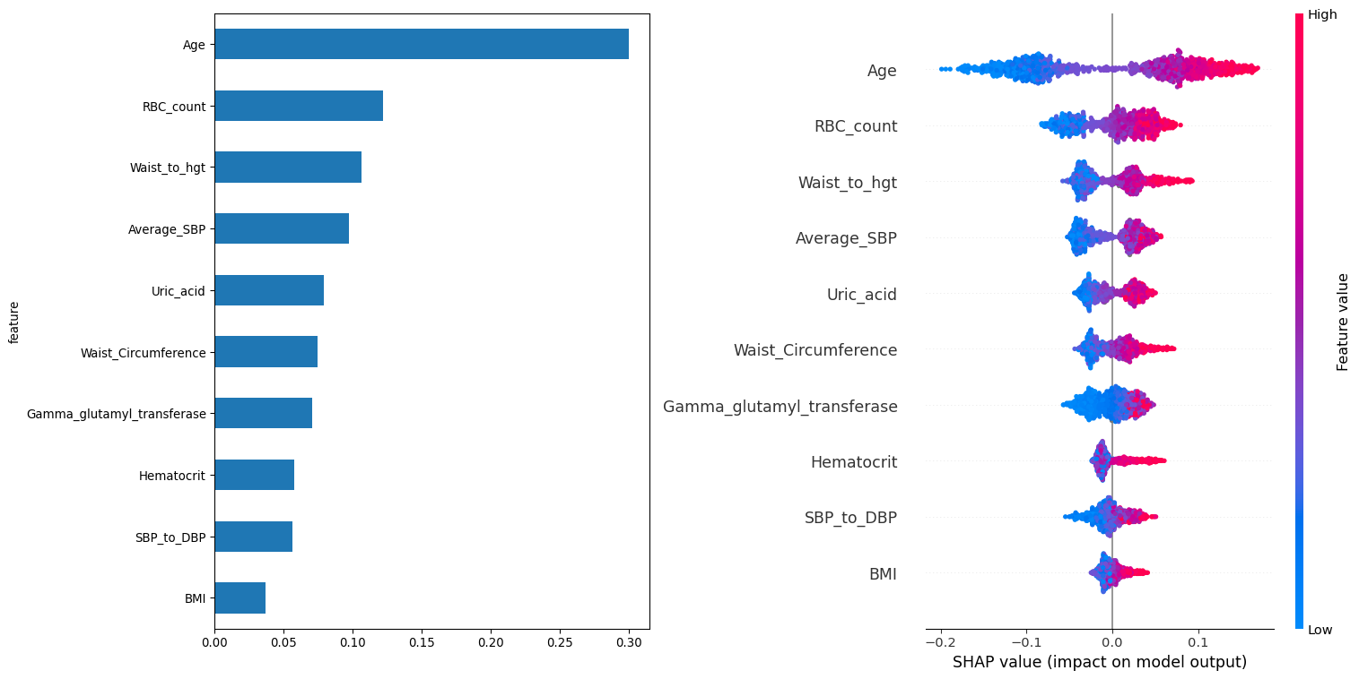
Based on the feature importance’s we can see the top five features are age, RBC count, waist to height ratio, average systolic blood pressure and waist circumference. Inspection of the SHAP value distributions does not provide any indication of a general direction of association for any features.
Synergy#
[18]:
# synergy heatmap
synergy_matrix = clf_inspector.feature_synergy_matrix()
MatrixDrawer(style="matplot%").draw(synergy_matrix, title="Feature synergies")
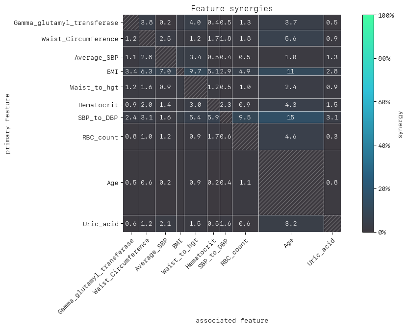
To interpret pairs of features in the synergy matrix, rows represent the primary feature (“perspective from”), and the columns represent associated features. Column and row widths indicate relative feature importance.
For example, for (SBP_to_DBP, RBC_count) from the perspective of primary feature SBP_to_DBP we find that 9.5% of its contribution to predict prediabetes risk is enabled by context from associated feature RBC_count, whereas RBC_count’s dependence on context from SBP_to_DBP is negligible.
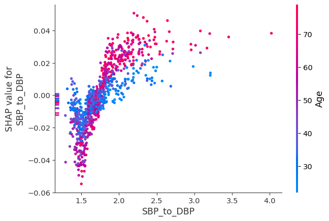
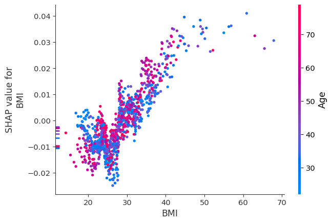
Another interesting observation is that looking at the column for Age from the perspective of other features such as BMI, RBC count and SBP_to_DBP, we see values ranging up to 15% suggesting that contributions of BMI, RBC count and SBP/DBP to predicting prediabetes are partly enabled by Age. By contrast, Age is a strong independent feature. It has the highest feature importance, as indicated by the column and row width of the matrix.
We can inspect synergistic pairs of features more deeply using the SHAP dependence plots offered by the SHAP package. The LearnerInspector provides all data required for creating these and other plots through method shap_plot_data():
[19]:
spd = clf_inspector.shap_plot_data()
shap.dependence_plot("SBP_to_DBP", spd.shap_values, spd.features, interaction_index="Age")
shap.dependence_plot("BMI", spd.shap_values, spd.features, interaction_index="Age")
Redundancy#
[20]:
# redundancy heatmap
redundancy_matrix = clf_inspector.feature_redundancy_matrix()
MatrixDrawer(style="matplot%").draw(redundancy_matrix, title="Feature redundancies")
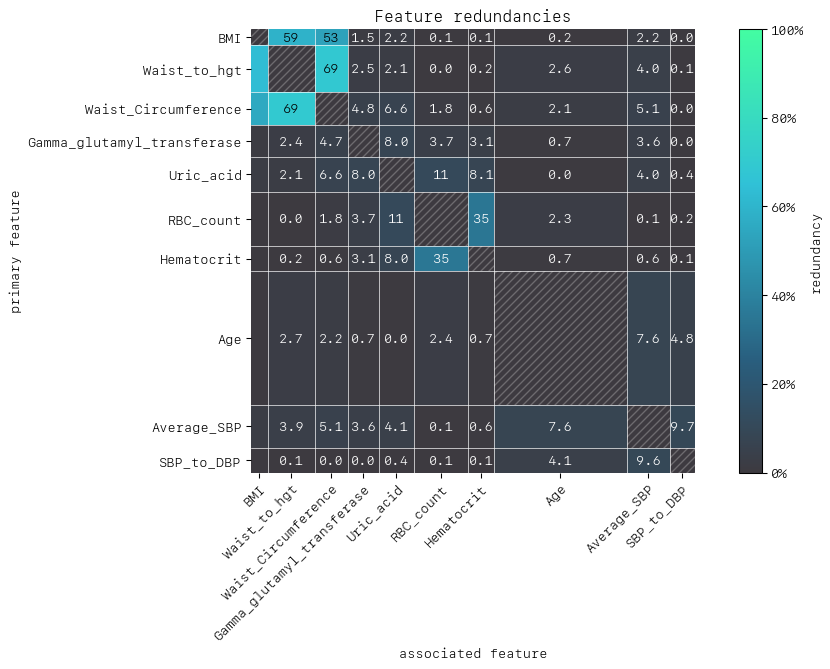
As with synergy, the matrix row is the primary feature (“perspective from”) in the row-column feature pair. Let’s take Hematocrit and RBC count as our features of interest. We can see that from the perspective of Hematocrit 35% of the information is duplicated with RBC count to predict prediabetes, and vice versa.
A second interesting and perhaps expected attribute of the heatmap is the apparent clustering of BMI, Waist Circumference and Waist/Height. Intuitively it makes sense that these features would have varying degrees of redundancy among them, given they are physically related.
Feature clustering#
As detailed above redundancy and synergy for a feature pair is from the “perspective” of one of the features in the pair, and so yields two distinct values. However, a symmetric version can also be computed that provides not only a simplified perspective but allows the use of (1 - metric) as a feature distance. With this distance, hierarchical, single linkage clustering is applied to create a dendrogram visualization. This helps to identify groups of low distance features which work “in tandem” to predict the outcome. Such information can then be used to either reduce clusters of highly redundant features to a subset or highlight clusters of highly synergistic features that should always be considered together.
For this example, let’s apply clustering to redundancy to see how the apparent grouping observed in the heatmap appears in the dendrogram. Ideally, we want to see features only start to cluster as close to the right-hand side of the dendrogram as possible. This implies all features in the model are contributing uniquely to our predictions.
[21]:
# redundancy dendrogram
dd_redundancy = clf_inspector.feature_redundancy_linkage()
DendrogramDrawer().draw(title="Redundancy linkage", data=dd_redundancy)
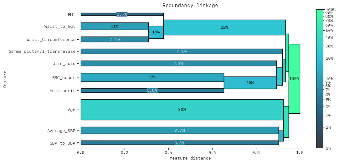
The dendrogram shows that Waist Circumference and Waist/Height cluster together first, which then cluster with BMI as well. This is a much clearer representation of the cluster of redundant features we observed in the heatmap. Considering BMI, Waist Circumference and Waist/Height:
What might we infer from synergy, redundancy and redundancy feature clustering?
BMI,Waist CircumferenceandWaist/Heightform a small cluster of redundant features. This seems reasonable:Waist Circumferenceis included in the calculation ofWaist/Heightwe might expect
BMIto capture similar information about excess body mass as higherWaist CircumferenceandWaist/Height
We saw little synergy between features. We might have expected apriori to find some interesting synergies between diet, exercise, sleep and body composition. Of course, the model needs to identify these relationships from them to be reflected in the synergy metric(s).
What action(s) might we take?
Given the redundancy that appears between BMI, Waist Circumference and Waist/Height, we could look to eliminate one or two of these features from the model.
For convenience when working in a non-notebook environment, all of the Drawer’s provided by the pytools package also support a style='text' flag.
[22]:
DendrogramDrawer(style="text").draw(title="Redundancy linkage", data=dd_redundancy)
============================== Redundancy linkage ==============================

BMI              4% ----------------------\
Waist_to_hgt    11% ------------------\___/---------------------------------\
Waist_Circumfer  7% ------------------/                                     |
Gamma_glutamyl_  7% -------------------------------------------------------\\
Uric_acid        8% -----------------------------------------------------\ ||__
RBC_count       12% ---------------------------------------\_____________/-/|
Hematocrit       6% ---------------------------------------/                |
Age             30% -------------------------------------------------------\|
Average_SBP     10% ------------------------------------------------------\//
SBP_to_DBP       6% ------------------------------------------------------/
Removing redundant features#
Recall the redundancy dendrogram above where we saw a clear cluster of features with redundancy; Waist/Height, BMI, and Waist Circumference.
assess if the features of the model are unique, i.e. not redundant with other features
decide which features to discard, combine, or modify to increase the uniqueness of important features in the model
Before we proceed to looking at SHAP values for individual predictions and perform a univariate simulation, let’s eliminate two partially redundant features - we will choose to keep Waist/Height ratio and drop BMI and Waist Circumference.
[23]:
# drop redundant features from our FACET sample object
prediab_no_redundant_feat = prediab_initial_features.drop(
    feature_names=["BMI", "Waist_Circumference"]
)
[24]:
clf_selector = LearnerSelector(
    searcher_type=RandomizedSearchCV,
    parameter_space=[rforest_ps, lgbm_ps],
    cv=RepeatedKFold(n_splits=5, n_repeats=10, random_state=42),
    n_jobs=-3,
    scoring="roc_auc",
    random_state=42,
).fit(prediab_no_redundant_feat)

clf_selector.summary_report()
[24]:
| score | candidate | param | time | ||||||||||
|---|---|---|---|---|---|---|---|---|---|---|---|---|---|
| test | - | classifier | fit | score | |||||||||
| rank | mean | std | - | max_depth | min_samples_leaf | n_estimators | min_child_samples | subsample | mean | std | mean | std | |
| 0 | 1 | 0.730649 | 0.033252 | RandomForestClassifierDF | 7 | 18 | 230 | NaN | NaN | 0.163255 | 0.011057 | 0.011816 | 0.005582 |
| 9 | 2 | 0.729762 | 0.033654 | RandomForestClassifierDF | 5 | 18 | 376 | NaN | NaN | 0.267629 | 0.019498 | 0.017950 | 0.007206 |
| 2 | 3 | 0.729191 | 0.032447 | RandomForestClassifierDF | 6 | 15 | 164 | NaN | NaN | 0.116502 | 0.003290 | 0.008389 | 0.000300 |
| 7 | 4 | 0.728881 | 0.033787 | RandomForestClassifierDF | 5 | 8 | 128 | NaN | NaN | 0.097372 | 0.010087 | 0.008520 | 0.003782 |
| 1 | 5 | 0.723997 | 0.034597 | RandomForestClassifierDF | 4 | 8 | 33 | NaN | NaN | 0.025100 | 0.000913 | 0.003405 | 0.000173 |
| 5 | 6 | 0.717630 | 0.029876 | LGBMClassifierDF | 4 | NaN | 58 | 9 | 0.922371 | 0.010459 | 0.000463 | 0.002328 | 0.000127 |
| 4 | 7 | 0.714231 | 0.031225 | LGBMClassifierDF | 5 | NaN | 37 | 8 | 0.860848 | 0.010239 | 0.000386 | 0.002252 | 0.000156 |
| 6 | 8 | 0.700294 | 0.031576 | LGBMClassifierDF | 7 | NaN | 78 | 8 | 0.891214 | 0.020512 | 0.000915 | 0.002845 | 0.000243 |
| 8 | 9 | 0.696527 | 0.032738 | LGBMClassifierDF | 4 | NaN | 167 | 8 | 0.834105 | 0.022742 | 0.004056 | 0.003137 | 0.001046 |
| 3 | 10 | 0.684973 | 0.032143 | LGBMClassifierDF | 6 | NaN | 379 | 8 | 0.966489 | 0.067832 | 0.001911 | 0.004945 | 0.000251 |
[25]:
# run inspector
inspector_no_redun = LearnerInspector(
    pipeline=clf_selector.best_estimator_,
    n_jobs=-3,
    verbose=False,
).fit(prediab_no_redundant_feat)
[26]:
# redundancy dendrogram
dd_redundancy = inspector_no_redun.feature_redundancy_linkage()
DendrogramDrawer().draw(title="HD set features", data=dd_redundancy)
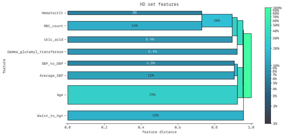
Now with the removal of BMI and Waist Circumference we can see the feature clustering starts much further to the right.
We can also check the best ranked model after removing redundant features.
[27]:
clf_selector.best_estimator_.classifier
[27]:
RandomForestClassifierDF(
    max_depth=7, min_samples_leaf=18, n_estimators=230, random_state=42
)
In a Jupyter environment, please rerun this cell to show the HTML representation or trust the notebook. On GitHub, the HTML representation is unable to render, please try loading this page with nbviewer.org.
RandomForestClassifierDF(
    max_depth=7, min_samples_leaf=18, n_estimators=230, random_state=42
)
FACET univariate simulator: the impact of waist to height ratio#
Another advantage of FACET is the ability to quickly instigate and run univariate simulation. Simulation enables us to gain insight into what value(s) of this ratio might minimize the likelihood of prediabetes.
As the basis for the simulation, we divide the feature into relevant partitions:
We use FACET’s
ContinuousRangePartitionerto split the range of observed values of waist to height ratio into intervals of equal size. Each partition is represented by the central value of that partition.For each partition, the simulator creates an artificial copy of the original sample assuming the variable to be simulated has the same value across all observations - which is the value representing the partition. Using the best estimator acquired from the selector, the simulator now re-predicts all targets using the models trained on full sample and determines the average value of the target variable resulting from this.
The FACET
SimulationDrawerallows us to visualise the result; both in a matplotlib and a plain-text style
[28]:
# set up and run a simulation
sim_feature = "Waist_to_hgt"

waist_to_hgt_simulator = UnivariateProbabilitySimulator(
    model=clf_selector.best_estimator_,
    sample=prediab_no_redundant_feat,
    n_jobs=-1,
)

waist_to_hgt_partitions = ContinuousRangePartitioner()

waist_to_hgt_simulation = waist_to_hgt_simulator.simulate_feature(
    feature_name=sim_feature,
    partitioner=waist_to_hgt_partitions
)
[29]:
# visualize the results
SimulationDrawer().draw(data=waist_to_hgt_simulation, title=sim_feature)
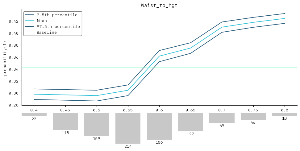
As we can see the simulation shows that higher waist to height ratios are associated with an increased risk of prediabetes. We could also suggest that keeping a person’s waist to height ratio below 0.52 may reduce the likelihood of prediabetes from around 34% to 30%.
[30]:
# can also get a print out of simulation results
SimulationDrawer("text").draw(data=waist_to_hgt_simulation, title=sim_feature)
================================= Waist_to_hgt =================================


probability(1):

Baseline = 0.342

Partition  2.5th percentile  Mean       97.5th percentile
=========  ================  =========  =================
0.4                0.289      0.297              0.306
0.45               0.287      0.296              0.305
0.5                0.286      0.295              0.304
0.55               0.295      0.304              0.313
0.6                0.352      0.361              0.37
0.65               0.366      0.375              0.383
0.7                0.401      0.409              0.418
0.75               0.409      0.417              0.426
0.8                0.416      0.424              0.432

Observed frequencies:

Partition  Frequency
=========  =========
0.4               22
0.45             118
0.5              159
0.55             214
0.6              186
0.65             127
0.7               69
0.75              46
0.8               18
Summary#
With the capabilities offered by FACET we were able to:
Identify a learner with performance comparable to models in the literature.
Utilize advanced the SHAP value capabilities (synergy and redundancy) to identify additional features that could be removed (i.e., BMI and waist circumference removed in favour of waist to height ratio) and whether any features had strong synergistic effects - which they did not.
Simulate the effect of changes in waist to height ratio on the likelihood of being prediabetic.
What can you do next?#
There are several next/alternative steps that could be taken:
Utilize methods to deal with class imbalance and see if it improves the model.
Adding more features! The NHANES data is a treasure trove of information.
Retain diabetic patients and convert it into a multi-class learning problem.
What would happen if we applied survey weights when constructing a learner?
Further investigation of feature engineering. One could also look at different sets of measurements such as the bio-profile and perform dimension reduction first via PCA or some other method.
Other learners such as SVC, LDA, Elastic-Net, CNN.
More sophisticated imputation for missing values: the assumption of MAR might not hold, as those with worse health and thus more at risk of prediabetes may be more likely not to disclose poor health characteristics. Methods enabled by IterativeImputer could be used or even KNNImputer. Also feature engineering could be done post imputation in the pipeline, so values such as ratios are consistent.
Appendix#
Data source and study cohort#
Instrument |
Data File Name (File) |
NHANES Field |
Description |
Dataset name |
Type |
|---|---|---|---|---|---|
Demographics |
Demographic Variables, Sample Weights (DEMO_H) |
RIDAGEYR |
Age in years at screening |
Age |
Numeric |
Demographics |
Demographic Variables, Sample Weights (DEMO_H) |
RIAGENDR |
Gender |
Gender |
Categorical |
Examination |
Body Measures (BMX_H) |
BMXWT |
Weight (kg) |
Weight |
Numeric |
Examination |
Body Measures (BMX_H) |
BMXHT |
Standing Height (cm) |
Standing_Height |
Numeric |
Examination |
Body Measures (BMX_H) |
BMXWAIST |
Waist Circumference (cm) |
Waist_Circumference |
Numeric |
Examination |
Body Measures (BMX_H) |
BMXBMI |
Body Mass Index (kg/m^2) |
BMI |
Numeric |
Examination |
Blood Pressure (BPX_H) |
BPXSY1 to 4 |
Systolic: Blood pres mm Hg |
Average_SBP |
Numeric |
Examination |
Blood Pressure (BPX_H) |
BPXDI1 to 4 |
Diastolic: Blood pres mm Hg |
Average_DBP |
Numeric |
Questionnaire |
Blood Pressure & Cholesterol (BPQ_H) |
BPQ020 |
Ever told you had high blood pressure |
High_BP |
Categorical |
Questionnaire |
Diet Behavior & Nutrition (DBQ_H) |
DBQ700 |
How healthy is the diet |
Healthy_diet |
Categorical |
Questionnaire |
Diabetes (DIQ_H) |
DIQ175A |
Family history |
Family_hist_diab |
Categorical |
Questionnaire |
Diabetes (DIQ_H) |
DIQ172 |
Feel could be at risk for diabetes |
Feel_at_risk_diab |
Categorical |
Questionnaire |
Current Health Status (HSQ_H) |
HSD010 |
General health condition |
General_health |
Categorical |
Questionnaire |
Medical Conditions (MCQ_H) |
MCQ080 |
Doctor ever said you were overweight |
Told_overweight |
Categorical |
Questionnaire |
Physical Activity (PAQ_H) |
PAQ605 |
Vigorous work activity |
Vigorous_work_activity |
Categorical |
Questionnaire |
Physical Activity (PAQ_H) |
PAQ620 |
Moderate work activity |
Moderate_work_activity |
Categorical |
Questionnaire |
Physical Activity (PAQ_H) |
PAQ635 |
Walk or bicycle |
Walk_or_bicycle |
Categorical |
Questionnaire |
Physical Activity (PAQ_H) |
PAQ650 |
Vigorous recreational activities |
Vigorous_rec_activity |
Categorical |
Questionnaire |
Physical Activity (PAQ_H) |
PAQ665 |
Moderate recreational activities |
Moderate_rec_activity |
Categorical |
Questionnaire |
Sleep Disorders (SLQ_H) |
SLD010H |
How much sleep do you get (hours)? |
Sleep_hours |
Numeric |
Questionnaire |
Sleep Disorders (SLQ_H) |
SLQ050 |
Ever told doctor had trouble sleeping? |
Trouble_sleeping |
Categorical |
Questionnaire |
Sleep Disorders (SLQ_H) |
SLQ060 |
Ever told by doctor have sleep disorder? |
Sleep_disorder |
Categorical |
Questionnaire |
Weight History (WHQ_H) |
WHQ070 |
Tried to lose weight in past year |
Tried_weight_loss_past_year |
Categorical |
Laboratory |
Cholesterol HDL (HDL_H) |
LBDHDD |
Direct HDL-Cholesterol (mg/dL) |
HDL_Cholesterol |
Numeric |
Laboratory |
Cholesterol Total (TCHOL_H) |
LBXTC |
Total Cholesterol(mg/dL) |
Total_Cholesterol |
Numeric |
Laboratory |
Complete Blood Count (CBC_H) |
LBXWBCSI |
White blood cell count (1000 cells/uL) |
WBC_count |
Numeric |
Laboratory |
Complete Blood Count (CBC_H) |
LBXRBCSI |
Red blood cell count (million cells/uL) |
RBC_count |
Numeric |
Laboratory |
Complete Blood Count (CBC_H) |
LBXHCT |
Haematocrit (%) |
Haematocrit |
Numeric |
Laboratory |
Biochemistry Profile (BIOPRO_H) |
LBXSTR |
Triglycerides (mg/dL) |
Triglycerides |
Numeric |
Laboratory |
Biochemistry Profile (BIOPRO_H) |
LBXSUA |
Uric acid (mg/dL) |
Uric_acid |
Numeric |
Laboratory |
Biochemistry Profile (BIOPRO_H) |
LBXSOSSI |
Osmolality (mmol/Kg) |
Osmolality |
Numeric |
Laboratory |
Biochemistry Profile (BIOPRO_H) |
LBXSNASI |
Sodium (mmol/L) |
Sodium |
Numeric |
Laboratory |
Biochemistry Profile (BIOPRO_H) |
LBXSKSI |
Potassium (mmol/L) |
Potassium |
Numeric |
Laboratory |
Biochemistry Profile (BIOPRO_H) |
LBXSGTSI |
Gamma glutamyl transferase (U/L) |
Gamma_glutamyl_transferase |
Numeric |
Laboratory |
Biochemistry Profile (BIOPRO_H) |
LBXSCA |
Total calcium (mg/dL) |
Calcium |
Numeric |
Laboratory |
Biochemistry Profile (BIOPRO_H) |
LBXSATSI |
Alanine aminotransferase ALT (IU/L) |
Alanine_aminotransferase |
Numeric |
Laboratory |
Biochemistry Profile (BIOPRO_H) |
LBXSASSI |
Aspartate aminotransferase AST (IU/L) |
Aspartate_aminotransferase |
Numeric |
Exploratory Data Analysis (EDA)#
Let’s begin by doing some brief exploratory data analysis to assess the impact features might have on the likelihood someone is prediabetic and to also determine what will need to be addressed in a preprocessing pipeline.
[31]:
# load the prepared data frame
prediab_eda = pd.read_csv("pre_diab_nhanes.csv")
prediab_eda.head()
[31]:
| Age | Gender | Waist_Circumference | Weight | Standing_Height | BMI | Average_SBP | Average_DBP | HDL_Cholesterol | Total_Cholesterol | ... | Triglycerides | Uric_acid | Osmolality | Sodium | Potassium | Gamma_glutamyl_transferase | Calcium | Alanine_aminotransferase | Aspartate_aminotransferase | Pre_diab | |
|---|---|---|---|---|---|---|---|---|---|---|---|---|---|---|---|---|---|---|---|---|---|
| 0 | 73.0 | 2.0 | NaN | 52.0 | 162.4 | 19.7 | 137.333333 | 86.666667 | 85.0 | 201.0 | ... | 88.0 | 4.2 | 290.0 | 142.0 | 4.1 | 31.0 | 10.0 | 28.0 | 36.0 | 1 |
| 1 | 56.0 | 1.0 | 123.1 | 105.0 | 158.7 | 41.7 | 157.333333 | 82.000000 | 38.0 | 226.0 | ... | 327.0 | 9.1 | 287.0 | 143.0 | 3.3 | 22.0 | 9.3 | 16.0 | 24.0 | 0 |
| 2 | 61.0 | 2.0 | 110.8 | 93.4 | 161.8 | 35.7 | 122.666667 | 80.666667 | 58.0 | 168.0 | ... | 68.0 | 5.1 | 281.0 | 140.0 | 3.9 | 17.0 | 9.9 | 21.0 | 20.0 | 1 |
| 3 | 56.0 | 2.0 | 85.5 | 61.8 | 152.8 | 26.5 | 122.000000 | 72.666667 | 59.0 | 278.0 | ... | 262.0 | 3.5 | 277.0 | 139.0 | 4.0 | 21.0 | 9.5 | 24.0 | 23.0 | 0 |
| 4 | 65.0 | 1.0 | 93.7 | 65.3 | 172.4 | 22.0 | 141.333333 | 77.333333 | 79.0 | 173.0 | ... | 39.0 | 6.3 | 281.0 | 140.0 | 4.8 | 24.0 | 9.5 | 20.0 | 29.0 | 0 |
5 rows × 38 columns
We might also consider some rudimentary feature engineering as well, such as the ratio of waist circumference to height or the ratio of systolic to diastolic blood pressure. Let’s create these two features as well.
[32]:
prediab_eda["SBP_to_DBP"] = prediab_eda["Average_SBP"] / prediab_eda["Average_DBP"]
prediab_eda["Waist_to_hgt"] = (
    prediab_eda["Waist_Circumference"] / prediab_eda["Standing_Height"]
)
prediab_eda.head()
[32]:
| Age | Gender | Waist_Circumference | Weight | Standing_Height | BMI | Average_SBP | Average_DBP | HDL_Cholesterol | Total_Cholesterol | ... | Osmolality | Sodium | Potassium | Gamma_glutamyl_transferase | Calcium | Alanine_aminotransferase | Aspartate_aminotransferase | Pre_diab | SBP_to_DBP | Waist_to_hgt | |
|---|---|---|---|---|---|---|---|---|---|---|---|---|---|---|---|---|---|---|---|---|---|
| 0 | 73.0 | 2.0 | NaN | 52.0 | 162.4 | 19.7 | 137.333333 | 86.666667 | 85.0 | 201.0 | ... | 290.0 | 142.0 | 4.1 | 31.0 | 10.0 | 28.0 | 36.0 | 1 | 1.584615 | NaN |
| 1 | 56.0 | 1.0 | 123.1 | 105.0 | 158.7 | 41.7 | 157.333333 | 82.000000 | 38.0 | 226.0 | ... | 287.0 | 143.0 | 3.3 | 22.0 | 9.3 | 16.0 | 24.0 | 0 | 1.918699 | 0.775677 |
| 2 | 61.0 | 2.0 | 110.8 | 93.4 | 161.8 | 35.7 | 122.666667 | 80.666667 | 58.0 | 168.0 | ... | 281.0 | 140.0 | 3.9 | 17.0 | 9.9 | 21.0 | 20.0 | 1 | 1.520661 | 0.684796 |
| 3 | 56.0 | 2.0 | 85.5 | 61.8 | 152.8 | 26.5 | 122.000000 | 72.666667 | 59.0 | 278.0 | ... | 277.0 | 139.0 | 4.0 | 21.0 | 9.5 | 24.0 | 23.0 | 0 | 1.678899 | 0.559555 |
| 4 | 65.0 | 1.0 | 93.7 | 65.3 | 172.4 | 22.0 | 141.333333 | 77.333333 | 79.0 | 173.0 | ... | 281.0 | 140.0 | 4.8 | 24.0 | 9.5 | 20.0 | 29.0 | 0 | 1.827586 | 0.543503 |
5 rows × 40 columns
[33]:
# first a quick look at features overall
prediab_eda.describe().T
[33]:
| count | mean | std | min | 25% | 50% | 75% | max | |
|---|---|---|---|---|---|---|---|---|
| Age | 4356.0 | 47.044536 | 17.188703 | 20.000000 | 33.000000 | 45.000000 | 61.000000 | 80.000000 |
| Gender | 4356.0 | 1.521350 | 0.499601 | 1.000000 | 1.000000 | 2.000000 | 2.000000 | 2.000000 |
| Waist_Circumference | 4158.0 | 97.167268 | 15.799909 | 55.500000 | 85.900000 | 95.500000 | 106.500000 | 177.900000 |
| Weight | 4321.0 | 79.939968 | 21.135093 | 32.300000 | 65.100000 | 76.900000 | 91.100000 | 222.600000 |
| Standing_Height | 4318.0 | 167.369701 | 10.158315 | 136.300000 | 160.000000 | 167.100000 | 174.500000 | 199.400000 |
| BMI | 4314.0 | 28.446639 | 6.793577 | 14.100000 | 23.700000 | 27.300000 | 31.800000 | 82.900000 |
| Average_SBP | 4229.0 | 121.893671 | 17.271841 | 64.666667 | 110.000000 | 118.666667 | 131.333333 | 228.000000 |
| Average_DBP | 4222.0 | 70.280515 | 11.039221 | 22.666667 | 63.333333 | 70.666667 | 77.333333 | 128.000000 |
| HDL_Cholesterol | 4318.0 | 53.723020 | 16.240125 | 10.000000 | 42.000000 | 51.000000 | 63.000000 | 173.000000 |
| Total_Cholesterol | 4318.0 | 190.363131 | 39.631288 | 69.000000 | 163.000000 | 188.000000 | 214.000000 | 525.000000 |
| High_BP | 4355.0 | 0.320321 | 0.466654 | 0.000000 | 0.000000 | 0.000000 | 1.000000 | 1.000000 |
| Sleep_hours | 4352.0 | 6.882812 | 1.389642 | 2.000000 | 6.000000 | 7.000000 | 8.000000 | 12.000000 |
| Trouble_sleeping | 4354.0 | 0.249426 | 0.432730 | 0.000000 | 0.000000 | 0.000000 | 0.000000 | 1.000000 |
| Sleep_disorder | 4346.0 | 0.085826 | 0.280139 | 0.000000 | 0.000000 | 0.000000 | 0.000000 | 1.000000 |
| Told_overweight | 4354.0 | 0.310978 | 0.462947 | 0.000000 | 0.000000 | 0.000000 | 1.000000 | 1.000000 |
| General_health | 4016.0 | 2.739293 | 0.952422 | 1.000000 | 2.000000 | 3.000000 | 3.000000 | 5.000000 |
| Family_hist_diab | 4356.0 | 0.219238 | 0.413778 | 0.000000 | 0.000000 | 0.000000 | 0.000000 | 1.000000 |
| Feel_at_risk_diab | 4311.0 | 0.288564 | 0.453147 | 0.000000 | 0.000000 | 0.000000 | 1.000000 | 1.000000 |
| Vigorous_work_activity | 4355.0 | 0.192652 | 0.394427 | 0.000000 | 0.000000 | 0.000000 | 0.000000 | 1.000000 |
| Moderate_work_activity | 4354.0 | 0.338769 | 0.473346 | 0.000000 | 0.000000 | 0.000000 | 1.000000 | 1.000000 |
| Walk_or_bicycle | 4356.0 | 0.254821 | 0.435811 | 0.000000 | 0.000000 | 0.000000 | 1.000000 | 1.000000 |
| Vigorous_rec_activity | 4356.0 | 0.246097 | 0.430785 | 0.000000 | 0.000000 | 0.000000 | 0.000000 | 1.000000 |
| Moderate_rec_activity | 4356.0 | 0.432277 | 0.495449 | 0.000000 | 0.000000 | 0.000000 | 1.000000 | 1.000000 |
| Tried_weight_loss_past_year | 3857.0 | 0.363495 | 0.481068 | 0.000000 | 0.000000 | 0.000000 | 1.000000 | 1.000000 |
| Healthy_diet | 4356.0 | 2.931359 | 0.995567 | 1.000000 | 2.000000 | 3.000000 | 4.000000 | 5.000000 |
| WBC_count | 4356.0 | 7.238522 | 2.313441 | 2.500000 | 5.700000 | 6.900000 | 8.400000 | 55.700000 |
| RBC_count | 4356.0 | 4.663620 | 0.482255 | 1.670000 | 4.347500 | 4.640000 | 4.970000 | 8.300000 |
| Hematocrit | 4356.0 | 41.543251 | 4.032086 | 17.900000 | 38.900000 | 41.500000 | 44.300000 | 55.900000 |
| Triglycerides | 4306.0 | 143.406410 | 105.113638 | 20.000000 | 76.000000 | 113.000000 | 176.000000 | 1213.000000 |
| Uric_acid | 4308.0 | 5.387303 | 1.384542 | 0.700000 | 4.400000 | 5.300000 | 6.300000 | 13.300000 |
| Osmolality | 4309.0 | 279.061963 | 4.825951 | 237.000000 | 276.000000 | 279.000000 | 282.000000 | 323.000000 |
| Sodium | 4309.0 | 139.882571 | 2.205999 | 119.000000 | 139.000000 | 140.000000 | 141.000000 | 154.000000 |
| Potassium | 4308.0 | 4.002948 | 0.347091 | 2.800000 | 3.800000 | 4.000000 | 4.200000 | 5.800000 |
| Gamma_glutamyl_transferase | 4308.0 | 27.459146 | 46.812967 | 5.000000 | 13.000000 | 18.000000 | 28.000000 | 1510.000000 |
| Calcium | 4289.0 | 9.451131 | 0.363228 | 7.600000 | 9.200000 | 9.400000 | 9.700000 | 14.800000 |
| Alanine_aminotransferase | 4307.0 | 24.831437 | 19.528176 | 6.000000 | 16.000000 | 20.000000 | 27.000000 | 536.000000 |
| Aspartate_aminotransferase | 4307.0 | 25.300906 | 19.612550 | 9.000000 | 19.000000 | 22.000000 | 27.000000 | 882.000000 |
| Pre_diab | 4356.0 | 0.346419 | 0.475883 | 0.000000 | 0.000000 | 0.000000 | 1.000000 | 1.000000 |
| SBP_to_DBP | 4222.0 | 1.765659 | 0.331493 | 1.272727 | 1.550097 | 1.684448 | 1.880256 | 5.470588 |
| Waist_to_hgt | 4152.0 | 0.581131 | 0.095154 | 0.364412 | 0.514059 | 0.571075 | 0.635716 | 1.063995 |
[34]:
# missingness
miss_count = prediab_eda.isna().sum()
miss_pct = miss_count[miss_count > 0] / len(prediab_eda)
miss_pct.sort_values().plot.barh()
[34]:
<AxesSubplot:>
[35]:
# those variables that are complete
miss_count[miss_count == 0] / len(prediab_eda)
[35]:
Age                      0.0
Gender                   0.0
Family_hist_diab         0.0
Walk_or_bicycle          0.0
Vigorous_rec_activity    0.0
Moderate_rec_activity    0.0
Healthy_diet             0.0
WBC_count                0.0
RBC_count                0.0
Hematocrit               0.0
Pre_diab                 0.0
dtype: float64
[36]:
# view correlations with a heatmap
df_cor = prediab_eda.corr()
sns.heatmap(df_cor, xticklabels=df_cor.columns, yticklabels=df_cor.columns)
[36]:
<AxesSubplot:>
[37]:
# let's do a table comparing features by the target

from tableone import TableOne

TableOne(
    prediab_eda,
    columns=prediab_eda.columns.drop("Pre_diab").to_list(),
    categorical=[
        "Gender",
        "High_BP",
        "Trouble_sleeping",
        "Sleep_disorder",
        "Told_overweight",
        "General_health",
        "Family_hist_diab",
        "Feel_at_risk_diab",
        "Vigorous_work_activity",
        "Moderate_work_activity",
        "Walk_or_bicycle",
        "Vigorous_rec_activity",
        "Moderate_rec_activity",
        "Tried_weight_loss_past_year",
        "Healthy_diet",
    ],
    groupby="Pre_diab",
    pval=True,
    remarks=False,
    overall=False,
)
[37]:
| Grouped by Pre_diab | |||||
|---|---|---|---|---|---|
| Missing | 0 | 1 | P-Value | ||
| n | 2847 | 1509 | |||
| Age, mean (SD) | 0 | 43.4 (16.4) | 54.0 (16.4) | <0.001 | |
| Gender, n (%) | 1.0 | 0 | 1330 (46.7) | 755 (50.0) | 0.040 |
| 2.0 | 1517 (53.3) | 754 (50.0) | |||
| Waist_Circumference, mean (SD) | 198 | 94.7 (15.3) | 101.9 (15.7) | <0.001 | |
| ... | ... | ... | ... | ... | ... |
| Calcium, mean (SD) | 67 | 9.5 (0.4) | 9.4 (0.4) | 0.129 | |
| Alanine_aminotransferase, mean (SD) | 49 | 24.0 (19.1) | 26.4 (20.2) | <0.001 | |
| Aspartate_aminotransferase, mean (SD) | 49 | 24.7 (14.1) | 26.5 (27.1) | 0.018 | |
| SBP_to_DBP, mean (SD) | 134 | 1.7 (0.3) | 1.8 (0.4) | <0.001 | |
| Waist_to_hgt, mean (SD) | 204 | 0.6 (0.1) | 0.6 (0.1) | <0.001 | |
61 rows × 4 columns
[38]:
# KDE plots by prediabetes status as well for those continuous features
distn_vars = [
    "Age",
    "Waist_Circumference",
    "Weight",
    "Standing_Height",
    "BMI",
    "Average_SBP",
    "Average_DBP",
    "HDL_Cholesterol",
    "Total_Cholesterol",
    "Sleep_hours",
    "WBC_count",
    "RBC_count",
    "Hematocrit",
    "Triglycerides",
    "Uric_acid",
    "Osmolality",
    "Sodium",
    "Potassium",
    "Gamma_glutamyl_transferase",
    "Calcium",
    "Alanine_aminotransferase",
    "Aspartate_aminotransferase",
    "SBP_to_DBP",
    "Waist_to_hgt",
]

df_kde = pd.melt(prediab_eda[distn_vars + ["Pre_diab"]], "Pre_diab", distn_vars)
g = sns.FacetGrid(
    df_kde, col="variable", hue="Pre_diab", col_wrap=5, sharex=False, sharey=False
)
g.map(sns.kdeplot, "value", fill=True)
plt.show()
Quick EDA summary:
Missingness
Our target and 10 features were complete.
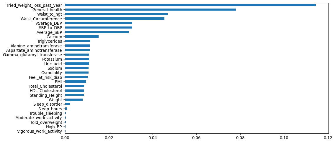
The other 29 features had levels of missing ranging from 0.02% to 11.5%, and 22 of the 29 were <3%.
Most extreme cases of missingness were for tried weight loss in the past year (11.5%) and general health (7.8%).
Correlations
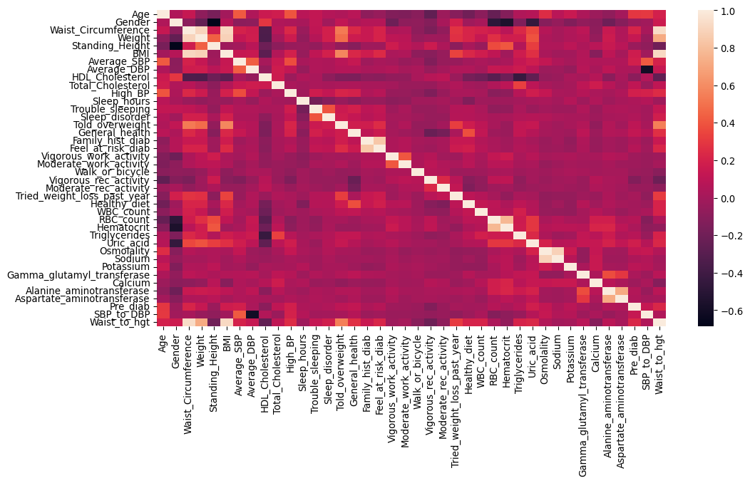
There is a wide range of correlation among features, where we can see that for example RBC count, haematocrit and standing height are all moderately negatively correlated with gender (i.e., females are shorter), and that body measurements for weight, height, BMI, and waist circumference are all strongly positively correlated.
Associations
Some features already appear to not to be strongly associated based on univariate tests, such as: average DBP, trouble sleeping, vigorous work activity, moderate work activity, tried weight loss in the past year, healthy diet, WBC count, and calcium levels.
Features associated with an increased risk of prediabetes include: older age, being male, increased waist circumference, decreased standing height, increased weight, increased BMI, increased average SBP, lower HDL cholesterol, increased total cholesterol, having high BP, increased sleep hours, having a sleep disorder, being told you are overweight, poorer general health, family history of diabetes, feeling at risk for diabetes, reduced walking or cycling, less vigorous or moderate recreational activity, higher RBC count, higher haematocrit, increased triglycerides, increased uric acid, higher osmolality, increased sodium, increased potassium, increased gamma glutamyl transferase, increased alanine aminotransferase, increased aspartate aminotransferase, increased SBP to DBP ratio, increased waist to height ratio.
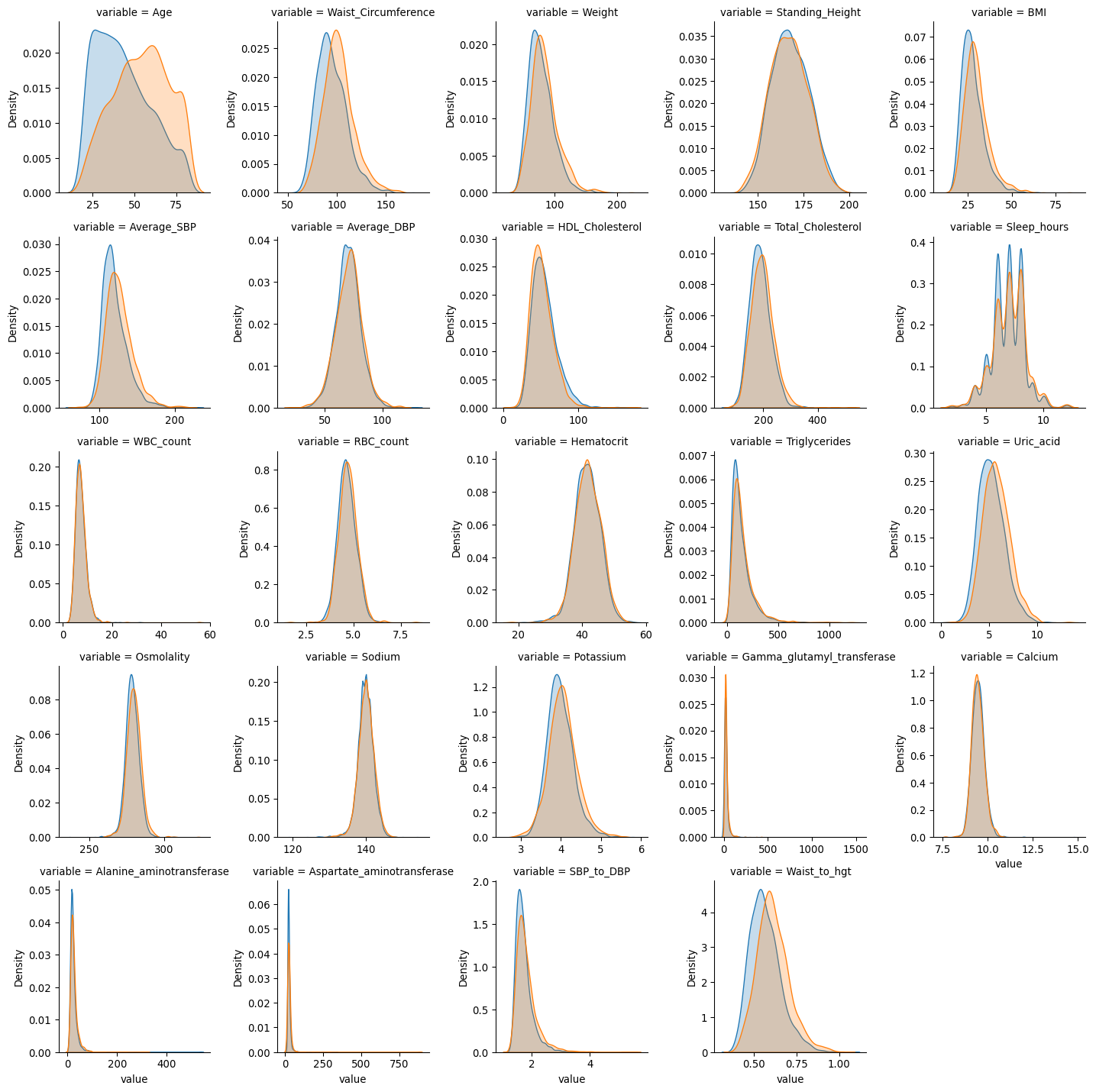
Distributions of numeric features
Many of the continuous features have been flagged as potentially non-normal/multi-modal and with potential outliers. This can be seen in the plots where many biomarkers have positive skewed distributions and in the case of sodium, some modality which could also be related to measurement.