Standard Scikit-learn Classification Summary with FACET

FACET is composed of the following key components:

• Model Inspection

  FACET introduces a new algorithm to quantify dependencies and interactions between features in ML models. This new tool for human-explainable AI adds a new, global perspective to the observation-level explanations provided by the popular SHAP approach. To learn more about FACET’s model inspection capabilities, see the getting started example below.

• Model Simulation

  FACET’s model simulation algorithms use ML models for virtual experiments to help identify scenarios that optimise predicted outcomes. To quantify the uncertainty in simulations, FACET utilises a range of bootstrapping algorithms including stationary and stratified bootstraps. For an example of FACET’s bootstrap simulations, see the getting started example below.

• Enhanced Machine Learning Workflow

  FACET offers an efficient and transparent machine learning workflow, enhancing scikit-learn’s tried and tested pipelining paradigm with new capabilities for model selection, inspection, and simulation. FACET also introduces sklearndf, an augmented version of scikit-learn with enhanced support for pandas dataframes that ensures end-to-end traceability of features.

---

Context

In this tutorial notebook we will first build a classifier for predicting customer churn using a well known datasets from Kaggle. Then using the developed classifier we will demonstrate how to perform selected typical model performance summary tasks including: - Using a final fitted model on all CV-folds to obtain a confusion matrix, classification report and precision-recall curve - Using models fitted to each CV fold, create a set of summary metrics and a ROC curve both with an assessment of error based on the cross-validation

---

Tutorial outline

1. Required imports

2. Quick data preparation

3. Preprocessing and feature selection

4. Learner selection with FACET

5. Using the final fitted model

6. Using the crossfit for the best model

In order to run this notebook, we will import not only the FACET package, but also other packages useful to solve this task. Overall, we can break down the imports into three categories:

1. Common packages (pandas, matplotlib, sklearn, etc.)

2. Required FACET classes (i.e., selection)

3. Other BCG GAMMA packages which simplify pipelining (sklearndf, see on GitHub) when using FACET

Common package imports

import numpy as np
import pandas as pd
from numpy import interp
import matplotlib.pylab as plt

from sklearn.metrics import (
    classification_report,
    confusion_matrix,
    roc_curve,
    roc_auc_score,
    auc,
    accuracy_score,
    f1_score,
    precision_score,
    recall_score,
    precision_recall_curve,
    ConfusionMatrixDisplay,
    PrecisionRecallDisplay,
)
from sklearn.compose import make_column_selector
from sklearn.model_selection import RepeatedKFold, GridSearchCV

FACET imports

from facet.data import Sample
from facet.selection import LearnerSelector, MultiEstimatorParameterSpace, ParameterSpace

sklearndf imports

Instead of using the “regular” scikit-learn package, we are going to use sklearndf (see on GitHub). sklearndf is an open source library designed to address a common issue with scikit-learn: the outputs of transformers are numpy arrays, even when the input is a data frame. However, to inspect a model it is essential to keep track of the feature names. sklearndf retains all the functionality available through scikit-learn plus the feature traceability and usability associated with Pandas data frames. Additionally, the names of all your favourite scikit-learn functions are the same except for DF on the end. For example, the standard scikit-learn import:

from sklearn.pipeline import Pipeline

becomes:

from sklearndf.pipeline import PipelineDF

from sklearndf.pipeline import PipelineDF, ClassifierPipelineDF
from sklearndf.classification import RandomForestClassifierDF
from sklearndf.transformation import (
    ColumnTransformerDF,
    OneHotEncoderDF,
    SimpleImputerDF,
)
from sklearndf.transformation.extra import BorutaDF

Quick data preparation

We start by obtaining a dataset for analysis. In this case we use the well known Telco Customer Churn dataset from Kaggle.

Briefly, the dataset contains one row for each of 7043 customers and includes information on those who left with the last month (i.e., Churn - our target of interest, n=1869), services signed up for, account information and demographics.

As this dataset has been well described and analyzed, we apply the minimum number of steps necessary to prepare the data for this tutorial. These are as follows:

• drop the customerID column

• convert TotalCharges to numeric type

• convert SeniorCitizen to string type

• relabel and convert Churn to a 0/1 target

Finally we place the dataframe in a FACET Sample object for easier data management. This allows us to:

• Quickly access the target vs. features

• Pass our data into sklearndf pipelines

• Pass information to other FACET functions

# This dataset is from Kaggle has been analyzed numerous times, and so we skip EDA
# read in the data
churn_df = pd.read_csv('KAGGLE-Telco-Customer-Churn.csv')

# drop customer ID
churn_df = churn_df.drop(columns=['customerID'])

# TotalCharges needs to be float (known to have a few missing values)
churn_df.TotalCharges = pd.to_numeric(churn_df.TotalCharges, errors='coerce')

# To support preprocessing pipeline we will also convert SeniorCitizen to object type
# only tenure, MonthlyCharges and TotalCharges are numeric
churn_df.SeniorCitizen = churn_df.SeniorCitizen.astype("category")

# Create a new 0/1 target where 1=churn
churn_df.Churn = churn_df.Churn.map(dict(Yes=1, No=0))

# create sample object
churn_sample = Sample(
    observations=churn_df,
    feature_names=churn_df.drop(columns=["Churn"]).columns,
    target_name="Churn",
)

print(f"churn sample data loaded with {len(churn_sample)} observations")

churn sample data loaded with 7043 observations

# get feature names
churn_sample.feature_names

['gender',
 'SeniorCitizen',
 'Partner',
 'Dependents',
 'tenure',
 'PhoneService',
 'MultipleLines',
 'InternetService',
 'OnlineSecurity',
 'OnlineBackup',
 'DeviceProtection',
 'TechSupport',
 'StreamingTV',
 'StreamingMovies',
 'Contract',
 'PaperlessBilling',
 'PaymentMethod',
 'MonthlyCharges',
 'TotalCharges']

Preprocessing and feature selection

Our first step is to create a minimum preprocessing pipeline which based on our dataset needs to address the following:

• Simple imputation for missing values

• One-hot encoding for categorical features

We will use the sklearndf wrappers for scikit-learn functions such as SimpleImputerDF in place of SimpleImputer, OneHotEncoderDF in place of OneHotEncoder, and so on.

# for categorical features we will use the mode as the imputation value and also one-hot encode
preprocessing_categorical = PipelineDF(
    steps=[
        ("imputer", SimpleImputerDF(strategy="most_frequent", fill_value="<na>")),
        ("one-hot", OneHotEncoderDF(sparse=False, handle_unknown="ignore")),
    ]
)

# for numeric features we will impute using the median
preprocessing_numerical = SimpleImputerDF(strategy="median")

# put the pipeline together
preprocessing_features = ColumnTransformerDF(
    transformers=[
        (
            "categorical",
            preprocessing_categorical,
            make_column_selector(dtype_include=object),
        ),
        (
            "numerical",
            preprocessing_numerical,
            make_column_selector(dtype_include=np.number),
        ),
    ],
    verbose_feature_names_out=False,
)

Next, we perform some initial feature selection using Boruta, a recent approach shown to have quite good performance. The Boruta algorithm removes features that are no more predictive than random noise. If you are interested further, please see this article.

The BorutaDF transformer in our sklearndf package provides easy access to this powerful method. The approach relies on a tree-based learner, usually a random forest. For settings, a max_depth of between 3 and 7 is typically recommended, and here we rely on the default setting of 5. However, as this depends on the number of features and the complexity of interactions one could also explore the sensitivity of feature selection to this parameter. The number of trees is automatically managed by the Boruta feature selector argument n_estimators="auto".

We also use parallelization for the random forest using n_jobs to accelerate the Boruta iterations.

# create the pipeline for Boruta
boruta_feature_selection = PipelineDF(
    steps=[
        ("preprocessing", preprocessing_features),
        (
            "boruta",
            BorutaDF(
                estimator=RandomForestClassifierDF(
                    max_depth=5, n_jobs=-3, random_state=42
                ),
                n_estimators="auto",
                random_state=42,
                verbose=False,
            ),
        ),
    ]
)

# run feature selection using Boruta and report those selected
boruta_feature_selection.fit(X=churn_sample.features, y=churn_sample.target)
selected = boruta_feature_selection.feature_names_original_.unique()
selected

array(['InternetService', 'OnlineSecurity', 'OnlineBackup',
       'DeviceProtection', 'TechSupport', 'StreamingTV',
       'StreamingMovies', 'Contract', 'PaperlessBilling', 'PaymentMethod',
       'tenure', 'MonthlyCharges', 'TotalCharges'], dtype=object)

Learner selection with FACET

FACET implements several additional useful wrappers which simplify comparing and tuning models:

• ParameterSpace: allows you to pass a learner pipeline (i.e., classifier + any preprocessing) and set hyperparameters.

• LearnerSelector: multiple LearnerGrids can be passed into this class as a list - this allows tuning hyperparameters both across different types of learners in a single step and ranks the resulting models accordingly

For the purpose of this tutorial we will assess a Random Forest Classifier and hyperparameter ranges will be assessed using 10 repeated 5-fold cross-validation and be scored using AUC:

Random forest: with hyperparameters

• max_depth: [4, 8, 16, 32]

• n_estimators: [200, 500]

Learner ranking uses the average performance minus two times the standard deviation, so that we consider both the average performance and variability when selecting a classifier.

If you want a list of available hyperparameters you can use classifier_name().get_params().keys() where classifier_name could be for example RandomForestClassifierDF and if you want to see the default values, just use classifier_name().get_params().

# reduce sample object to selected features
churn_sample_kept_features = churn_sample.keep(feature_names=selected)

# Classifier pipeline composed of the feature preprocessing steps created earlier and random forest learner
rforest_clf = ClassifierPipelineDF(
    preprocessing=preprocessing_features,
    classifier=RandomForestClassifierDF(random_state=42),
)

# set space of hyper-parameters
classifier_ps = ParameterSpace(rforest_clf)
classifier_ps.classifier.max_depth = [4, 7, 10]
classifier_ps.classifier.n_estimators = [100, 200]

# run the learner selector
clf_selector = LearnerSelector(
    searcher_type=GridSearchCV,
    parameter_space=classifier_ps,
    cv=RepeatedKFold(n_splits=5, n_repeats=10, random_state=42),
    n_jobs=-3,
    scoring="roc_auc",
).fit(churn_sample_kept_features)

# look at results
clf_selector.summary_report()

	score			param		time
	test			classifier		fit		score
	rank	mean	std	max_depth	n_estimators	mean	std	mean	std
3	1	0.846467	0.010198	7	200	0.428813	0.005649	0.030035	0.002274
2	2	0.846176	0.010207	7	100	0.225023	0.002987	0.018026	0.000395
1	3	0.842705	0.010570	4	200	0.330742	0.004208	0.022932	0.000563
0	4	0.842060	0.010702	4	100	0.176152	0.002248	0.014863	0.000459
5	5	0.841639	0.010050	10	200	0.548096	0.022182	0.038036	0.003584
4	6	0.840989	0.010235	10	100	0.288122	0.019839	0.023028	0.003089

Using the final fitted model

As part of the clf_selector we can access a final model (best_estimator_) that represents the selected best model but re-fit using all available training data. With this model we can then predict either the class or the probability (score) and generate standard scikit-learn classifier performance summaries such as a classification report, confusion matrix or precision-recall curve.

# obtain required quantities
y_pred = clf_selector.best_estimator_.predict(churn_sample_kept_features.features)
y_prob = clf_selector.best_estimator_.predict_proba(churn_sample_kept_features.features)[1]
y_true = churn_sample_kept_features.target

Classification Report

The classification report from scikit-learn is often used as a summary for classifiers, especially in the case of imbalanced datasets, as it provides precision, recall and the f1-score by class along with the support (number of observations for a class). For more information on the implementation in scikit-learn please see sklearn.metrics.classification_report.

print(classification_report(y_true, y_pred))

              precision    recall  f1-score   support

           0       0.84      0.92      0.88      5174
           1       0.70      0.53      0.61      1869

    accuracy                           0.82      7043
   macro avg       0.77      0.73      0.74      7043
weighted avg       0.81      0.82      0.81      7043

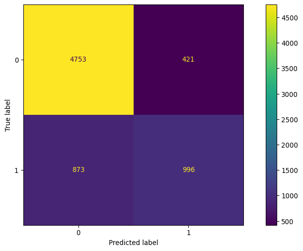
Confusion Matrix

The confusion matrix can be used to evaluate the accuracy of the fitted classifier by comparing the predicted class to the observed class. For more information on the implementation in scikit-learn please see sklearn.metrics.confusion_matrix.

cf_matrix = confusion_matrix(y_true, y_pred)
ConfusionMatrixDisplay(cf_matrix).plot()

<sklearn.metrics._plot.confusion_matrix.ConfusionMatrixDisplay at 0x1491a55b0>

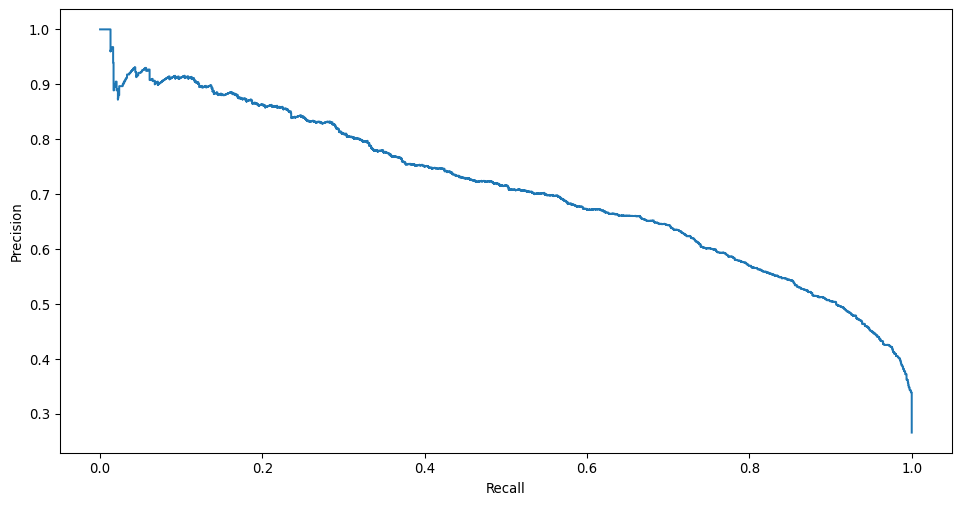
Precision-recall curve

The precision-recall curve is helpful for understanding the trade off between precision (positive predictive value) and recall (sensitivity) according to a specified threshold applied to the predicted probability (or score) for determining the predicted class for an observation. For more information on the implementation in scikit-learn please see sklearn.metrics.precision_recall_curve.

prec, recall, _ = precision_recall_curve(y_true, y_prob, pos_label=1)
PrecisionRecallDisplay(precision=prec, recall=recall).plot()

<sklearn.metrics._plot.precision_recall_curve.PrecisionRecallDisplay at 0x14951d8e0>

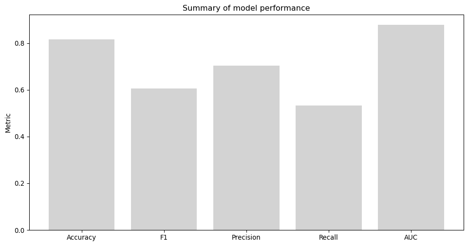
Panel of metrics

Below we demonstrate how to use the best estimator results to obtain a set of common classification metrics: Accuracy, F1, Precision, Recall and AUC. This approach can of course be adapted to any metric and any summary thereof.

For more information about classifier metrics in scikit-learn please see classification-metrics.

metrics = []

# calculate metrics
metrics.append(pd.Series({
    'Accuracy': accuracy_score(y_true, y_pred),
    'F1': f1_score(y_true, y_pred),
    'Precision': precision_score(y_true, y_pred),
    'Recall': recall_score(y_true, y_pred),
    'AUC': roc_auc_score(y_true, y_prob)})
)

# collect required summaries and plot
metrics_df = pd.DataFrame(metrics)
fig, ax = plt.subplots()
ax.bar(
    metrics_df.columns,
    metrics_df.mean(),
    align='center',
    ecolor='lime',
    capsize=10,
    color='lightgrey'
)
ax.set_ylabel('Metric')
ax.set_title('Summary of model performance')

Text(0.5, 1.0, 'Summary of model performance')

previous

Classification with FACET: Prediabetes Study

next

Development Guidelines